NAMD Tutorial: Molecular Dynamics of Na+/Cl- Association
by Karl Debiec and Ali Saglam
Updated with WESTPA version 1.0 beta and NAMD 2.1.0
Overview
Requirements: ~3 hr wallclock time on an 8-core Intel Westmere node (one walker per core); ~1.3 GB disk space
In this tutorial we will use the standard weighted ensemble approach to simulate Na+/Cl- association in Generalized Born implicit solvent. The system consists of single Na+ and Cl- ions modeled with the CHARMM force field, using the distance between the two ions as the progress coordinate. NAMD will be used to run the molecular dynamics, and familiarity with it is a prerequisite (see tutorials). Basic knowledge of python and bash scripting is also necessary.
The first step is to set up a directory containing the necessary NAMD and
WESTPA files. A working example directory can be found at
westpa/lib/examples/nacl_namd.
Preparing the NAMD files
| Input File | Description |
|---|---|
| nacl.psf | topology |
| nacl.pdb | coordinates |
| md-genvel.conf | NAMD configuration for initial segments |
| md-continue.conf | NAMD configuration for continuations |
| par_all27_prot_na.prm | force field parameters |
The above files are included in the namd_config subfolder of the example
directory, and should be familiar to NAMD users. Note that two configuration
files are present.
md-genvel.conf is used for initial segments, in which it is necessary to
generate initial velocities, and md-continue.conf is used for
continuations, in which velocities are inherited from the parent segment.
md-continue.conf
#   0.5 ps NVT production with Langevin thermostat and GB implicit solvent
#################################### INPUT ####################################
paraTypeCharmm  on                      ;# Parameter infile  in 'CHARMM' format
coordinates     parent.coor             ;# Structure infile
velocities      parent.vel              ;# Velocity infile
structure       nacl.psf                ;# Topology infile
parameters      par_all27_prot_na.prm   ;# Parameter infile
seed            RAND                    ;# Use random seed from WESTPA
################################## ENSEMBLE ###################################
langevin        on        ;# Langevin thermostat enabled
temperature     300       ;# Initial temperature (K)
langevindamping 0.5       ;# Thermostat damping constant (ps -1)
########################### NONBONDED INTERACTIONS ############################
cutoff          999.0     ;# Nonbonded cutoff
exclude         scaled1-4 ;# Scaling between 1-4 bonded atoms
1-4scaling      1.0       ;# 1-4 interaction scaling
switching       off       ;# Van der Waals switching disabled
pairlistdist    1000.0    ;# Neighbor list cut-off (A)
stepspercycle   250       ;# Neighbor list update interval (timesteps)
############################## IMPLICIT SOLVENT ###############################
GBIS            on        ;# Generalized Born implicit solvent
################################### OUTPUT ####################################
outputname      seg       ;# Output file prefix
outputEnergies  50        ;# Energy log output interval (timesteps)
restartfreq     0         ;# Restart file output interval (timesteps)
binaryoutput    no        ;# Do not output binary trajectory
dcdfile         seg.dcd   ;# Trajectory outfile
dcdfreq         50        ;# Trajectory output interval (timesteps)
################################# INTEGRATOR ##################################
timestep        2.0       ;# Simulation timestep (fs)
run             250       ;# Simulation duration (timesteps)
Several settings in this configuration file are important to WESTPA. First is the the segment duration, τ, which is equal to the timestep times the number of steps. The appropriate τ depends on the system and progress coordinate, and for this system we have chosen 0.5 ps. Second is the use of the stochastic Langevin thermostat; WESTPA requires a stochastic element such that trajectories branched from a common point diverge. In order to ensure that this occurs, it is also necessary to set the random seed to a different value for each segment. Setting the random seed based on the time, as is common for brute-force simulations, may cause problems as simulations started simultaneously from the same parent will not diverge.
NAMD configuration files support tcl scripting, which we use to export each frame of the trajectory after dynamics have been run.
md-continue.conf (continued)
################################### OUTPUT ####################################
coorfile open dcd seg.dcd
set i 0
while { ![coorfile read] } {
    output [format "%04d" [expr $i]]
    set i [expr $i + 1]
}
This allows us to read the coordinates for each frame in bash without relying on an external program such as Visual Molecular Dynamics. This is done for this tutorial to avoid dependence on other software; in production simulations it is preferable to use faster methods.
The analogous md-genvel.conf differs only in that it does not load
velocities from the input file, instead generating them from a Maxwellian
distribution.
Preparing the WESTPA files
| Input File | Description |
|---|---|
| env.sh | set environment variables |
| gen_istate.sh | generate initial states from basis states |
| get_pcoord.sh | calculate progress coordinate for initial states |
| system.py | system implementation |
| runseg.sh | segment implementation |
| post_iter.sh | post-segment cleanup |
| west.cfg | WESTPA configuration |
| init.sh | initialize WESTPA |
| run.sh | run WESTPA |
| tar_segs.sh | tar segments |
The above files are listed roughly in the order in which it is appropriate to
configure them. gen_istate.sh, get_pcoord.sh, runseg.sh, and
post_iter.sh are located in the westpa_scripts subfolder.
env.sh
This script sets environment variables that may be used across the simulation. These include the root directory for WESTPA, the root directory for the simulation, the name for the simulation, and the python executable to use. It also sets the executable for NAMD; using an environment variable for this purpose makes it easier to transition code to different hardware or test different builds or flags of an MD code without editing multiple files.
gen_istates.sh
This script generates initial states (structures) for the simulation from the
basis states (structures) stored in the bstates subfolder. Our system
contains a single basis state containing the two ions with a separation of 9.90
Å; this script generates slight variations of this distance in order to obtain
a greater variety of starting configurations.
get_pcoord.sh
This script calculates the progress coordinate from the initial states. Our
progress coordinate is the distance between the Na+ and Cl-
ions; since it is very simple, we may calculate it using only shell commands.
Note that this script is used only during initial state generation; during
production runseg.sh calculates the progress coordinate.
system.py
This file contains the python implementation of this WESTPA system. Here are
specified the number of dimensions in the progress coordinate, the number of
frames to be output per segment, the bin boundaries, and the number of walkers
per bin. For this system we use 22 bins as defined by Zwier, Kaus, and Chong, and 24 walkers per bin.
system.py also includes the functions coord_loader and log_loader.
In addition to the progress coordinate, WESTPA includes the ability to
calculate and store auxiliary data as the simulation is run. This is often
easier than looping over iterations and segments afterwards. Since our system
contains only two atoms, it is reasonable for us to store all coordinate
information in the same hdf5 file as the progress coordinate. We will also
store the log information including time, energy, and temperature.
runseg.sh
This script runs individual segments, calculates and outputs their progress
coordinates, and outputs auxiliary data. For each iteration and segment it
generates a folder, linking to the files necessary for running NAMD.
For the NAMD configuration file, it uses sed to input a random seed
generated by WESTPA. It then runs NAMD, calculates and outputs the progress
coordinate and auxiliary data, and removes files that are no longer needed. As
in get_pcoord.sh, the progress coordinate is calculated using shell
commands.
The auxiliary coordinate dataset is prepared using the coor files output by
NAMD, which are processed using shell commands and output to a temporary file,
from which it is read by the coord_loader function in system.py.
The auxiliary log data is similarly processed using shell commands and output
to a temporary file, from which it is read by the log_loader function in
system.py.
post_iter.sh
This script cleans up after each iteration. WESTPA simulations can generate
large numbers of files, potentially conflicting with filesystem restrictions.
After each iteration, post_iter.sh moves the segment logs the associated
segment logs to a tar file.
west.cfg
This file contains the WESTPA configuration, including the locations of various scripts and the nature of the anticipated output. Additionally, this is where the number of iterations and maximum production time are set. Some optional functions, such as the ability to run a designated script before each iteration, are listed but unused in this tutorial.
init.sh
This script initializes the WESTPA system. It removes files from previous runs
and uses gen_istates.sh and get_pcoord.sh to generate initial states. This
is also where the basis states and target states are defined. For this system
we define the bound target state as 1.8 Å separation, and the unbound target
state as 16.9 Å separation. Once walkers reach the bins containing these values
(i.e. our first and final bins), they are recycled. init.sh is also one of
two places where we specify the number of walkers per bin, as
--segs-per-state.
run.sh
This script is used to run WESTPA.
tar_segs.sh
This script is used to tar segments after the WESTPA simulation has been run,
in order to reduce the number of files produced. In order to allow extension of
the simulation, the last segment is not tarred. Typically, it is advisable not
to tar segments after each iteration (i.e. in post_iter.sh), while the main
WESTPA process is tarring, other cores are idle, potentially wasting CPU time.
Running the simulation
From the simulation root directory ($WEST_SIM_ROOT), the simulation may be
initialized using the command:
./init.sh
and run using the command:
./run.sh
init.sh and run.sh call w_init and w_run from WESTPA. By
default WESTPA will use as many cores as are available on the host machine. If
the simulation is run on a computing cluster, w_run may be executed from
a batch script. See the Running page for more information on how to
submit jobs to specific clusters.
Analyzing the data
Output
| Output File | Remarks |
|---|---|
| traj_segs | output from each iteration and segment |
| seg_logs | log files from each iteration and segment |
| west.h5 | WESTPA output in hdf5 database |
| west.log | WESTPA log file |
traj_segs
This folder stores the results of the WESTPA simulation, organized by iteration
and segment. This includes all files generated by runseg.sh, including
those generated by NAMD.
For this system, the only files saved are seg.coor, seg.vel, and
seg.log corresponding to the coordinates, velocities, and log.
After the simulation has been run, tar_segs.sh may be used to reduce each
iteration to a single tar file.
seg_logs
This folder stores logs from each iteration and segment. post_iter.sh has
been used to combine each segment into a single tar file.
west.h5
This file stores the simulation output in an hdf5 database. This includes the relationships between successive walkers, bin weights, progress coordinates, and auxiliary data.
west.log
This file contains a brief log of simulation progress. As WESTPA runs, it outputs information such as the current iteration number, the number of populated bins, and the time needed for each iteration in this log. This is also where errors are output.
Since only 10 iterations have been run, we do not yet have enough data to
analyze. Edit west.cfg and change max_total_iterations to 100. Extend
using the command:
./run.sh
Computing the association rate
WESTPA includes several tools for analysis located in $WEST_ROOT/bin. In
init.sh we specified the bin containing an Na+/Cl-
distance of 1.8 Å as the bound state, and that containing a distance of 16.9 Å
as the unbound state. Using w_fluxanl, we can calculate the flux into these
target states, and from that calculate the association rate of Na+/Cl-. w_fluxanl may be run with the following commands:
source env.sh
$WEST_ROOT/bin/w_fluxanl
The script will output the flux into the target states including confidence intervals calculated using the block bootstrap method:
Calculating mean flux and confidence intervals for iterations [1,101)
target 'unbound':
  correlation length = a tau
  mean flux and CI   = b (c, d) tau^(-1)
target 'bound':
  correlation length = w tau
  mean flux and CI   = x (y, z) tau^(-1)
More information on how to use w_fluxanl can be viewed using the --help
flag. w_fluxanl also stores this information in an hdf5 file,
fluxanl.h5. Using the python libraries h5py and pylab, we can visualize
this data. Open a python interpreter and run the following commands:
import h5py, numpy, pylab
fluxanl              = h5py.File('fluxanl.h5')
flux                 = numpy.zeros(100)
first_binding        = 100 - fluxanl['target_flux']['target_1']['flux'].shape[0]
flux[first_binding:] = numpy.array(fluxanl['target_flux']['target_1']['flux'])
pylab.plot(flux)
pylab.xlabel("Iteration")
pylab.ylabel("Instantaneous Flux $(\\frac{1}{\\tau})$")
pylab.show()
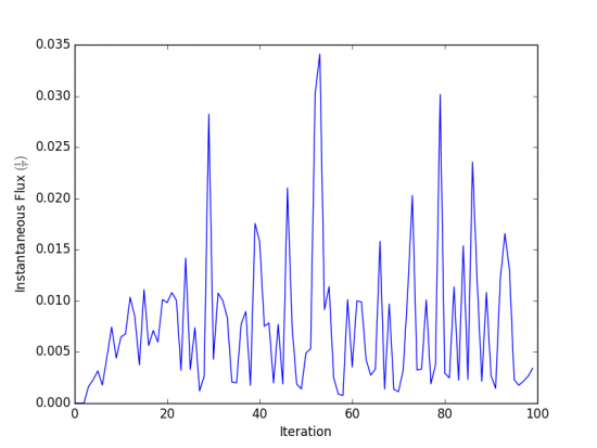
The x-axis represents the iteration number, and the y-axis the flux into the
bound state in units of τ-1 during that iteration. In the above
simulation, the first transition to the unbound state occurred in iteration 2,
and the first transition to the bound state occurred in iteration 3. The
instantaneous flux is noisy and difficult to interpret, and it is clearer to
view the time evolution of the flux. Run w_fluxanl again, this time with
the --evol flag:
$WEST_ROOT/bin/w_fluxanl --evol
We may plot the time evolution of flux using the following commands at a python interpreter:
import h5py, numpy, pylab
fluxanl   = h5py.File('fluxanl.h5')
mean_flux = numpy.zeros(100)
ci_ub     = numpy.zeros(100)
ci_lb     = numpy.zeros(100)
first_binding             = 100 - fluxanl['target_flux']['target_1']['flux_evolution']['expected'].shape[0]
mean_flux[first_binding:] = numpy.array(fluxanl['target_flux']['target_1']['flux_evolution']['expected'])
ci_lb[first_binding:]     = numpy.array(fluxanl['target_flux']['target_1']['flux_evolution']['ci_lbound'])
ci_ub[first_binding:]     = numpy.array(fluxanl['target_flux']['target_1']['flux_evolution']['ci_ubound'])
pylab.plot(mean_flux, 'b', ci_lb, 'g', ci_ub, 'r')
pylab.xlabel("Iteration")
pylab.ylabel("Mean Flux $(\\frac{1}{\\tau})$")
pylab.show()
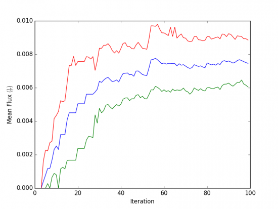
We can see that the flux has plateaued, indicating that the simulation has reached steady-state conditions. When calculating the rate, we discard the portion of data during which the system is equilibrating, using only portion over which the rates are steady and converging. We may calculate the rate using only the last 50 iterations:
$WEST_ROOT/bin/w_fluxanl --first-iter 50

Calculating mean flux and confidence intervals for iterations [50,101)
target 'unbound':
  correlation length = 1 tau
  mean flux and CI   = 1.268496e-01 (1.179945e-01,1.355673e-01) tau^(-1)
target 'bound':
  correlation length = 0 tau
  mean flux and CI   = 7.917146e-03 (5.870760e-03,1.014573e-02) tau^(-1)
Your output should be within an order of magnitude. Since τ for our simulation
was 0.5 ps, in order to determine the association rate in units of ps-1, the flux should be multiplied by 2, giving an association rate of
1.6 x 10⁻² ps-1 with a 95% CI of 1.2 x10⁻² to 2.0
x10-2. In order to obtain a more precise association rate, we would
need to run more iterations of the simulation, which may be done by editing
west.cfg.
Visualizing a selected pathway
Westpa includes the tools w_succ and w_trace to make concatenating
the segments for one of your completed pathways straightforward. Both
w_succ and w_trace are located in $WEST_ROOT/bin.
First use w_succ by entering into the command line from your simulation
root directory:
source env.sh
$WEST_ROOT/bin/w_succ
w_succ will output a list of every completed pathway, listed by its
iteration and segment ids. The target state each pathway has reached may be
determined from the final value of the progress coordinate. Pick any set of
completed iteration and segment ids and use them with the w_trace tool.
For example, if iteration 17 segment 2 is a completed pathway, run:
$WEST_ROOT/bin/w_trace 17:2
w_trace will output a text file named traj_17_2_trace.txt listing the
iteration and segment ids for the chain of continuing segments leading up to
the successful completion of your simulation. This file includes the iteration,
seg_id, weight, wallclock time, CPU time, and final progress coordinate value
for each segment comprising the trajectory. The first line, listed as iteration
0, includes the initial state ID. The same information is stored in hdf5 format
in the outfile trajs.h5.
By combining the information in this file with the coordinates stored in
west.h5, we can generate a complete trajectory viewable using Visual
Molecular Dynamics using the script
cat_trajectory.py, included in the westpa_scripts subfolder:
import h5py, numpy, sys

infile = numpy.loadtxt(sys.argv[1], usecols = (0, 1))
west   = h5py.File('west.h5')
coords = []
for iteration, seg_id in infile[1:]:
    iter_key = "iter_{0:08d}".format(int(iteration))
    SOD      = west['iterations'][iter_key]['auxdata']['coord'][seg_id,1:,0,:]
    CLA      = west['iterations'][iter_key]['auxdata']['coord'][seg_id,1:,1,:]
    coords  += [numpy.column_stack((SOD, CLA))]
with open(sys.argv[1][:-4] + ".xyz", 'w') as outfile:
    for i, frame in enumerate(numpy.concatenate(coords)):
        outfile.write("2\n")
        outfile.write("{0}\n".format(i))
        outfile.write("SOD {0:9.5f} {1:9.5f} {2:9.5f}\n".format(
          float(frame[0]), float(frame[1]), float(frame[2])))
        outfile.write("CLA {0:9.5f} {1:9.5f} {2:9.5f}\n".format(
          float(frame[3]), float(frame[4]), float(frame[5])))
This script takes w_trace output as a command line argument, loads the
iteration and segment IDs, loads the coordinates for each segment from
west.h5`, and saves the results into an xyz file viewable using VMD.
Useful links
Useful hints
- Make sure your paths are set correctly in
env.sh - If the simulation doesn’t stop properly with CTRL+C , use CTRL+Z.
- Another method to stop the simulation relatively cleanly is to rename
runseg.sh; WESTPA will shut the simulation down and prevent the hdf5 file from becoming corrupted. Some extra steps may be necessary to ensure that the analysis scripts can be run successfully.
